Analyzing Angular Correlations¶

While angular correlations can be easily (and quickly calculated) they are highly susceptible to even small misalignment in the microscope. Additionally, thick samples which are more dominated by dynamical scattering, render the data collected largely useless.

Starting with the equation for the angular correlation is given by:

$C(\phi,k,n)= \frac{ <I(\theta,k,n)*I(\theta+\phi,k,n)>_\theta-<I(\theta,k,n)>^2}{<I(\theta,k,n)>^2}$

Where $\theta$ is the entire $2\pi$ radians the that $\phi$ (the angle of correlation) is averaged over. k is the radius of the reciporical space vector and n is the diffraction pattern number (assuming the correlation is being calculated for a series of diffraction patterns)

While the Electron Microscope community has decided to use the terminology of angular correlations, what is being calculated is in actuality the self-correlation as a function of angle instead of time.

As result efficient methods for convolution can be applied in which the actual computation occurring is:

$C(\phi,k,n)=\frac{IFFT[FFT(I(\theta,k,n))_\theta * Conj(FFT(I(\theta,k,n)))_\theta]}{<I(\theta,k,n)>^2}$

Which speeds up the calculation more than 100x

Calculating the Angular Correlations

In order to calculate angular correlations, start by loading a 4-D data set.

import hyperspy.api as hs
import matplotlib.pyplot as plt

dif_signal = hs.load(file, signal_type ='diffraction_signal')

# adding a mask to the signal for to block the beam stop
dif_signal.mask_below(.1)
dif_signal.show_mask()

# correcting for not elliptical diffraction patterns. Make sure there is not wobbling from pattern to pattern
dif_signal.determine_ellipse()
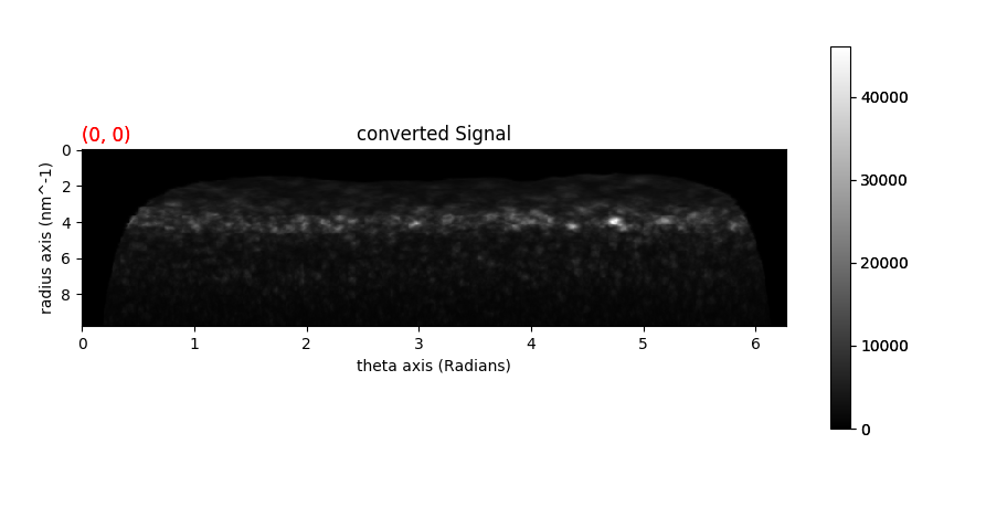
pol_signal = dif_signal.calculate_polar_spectrum()
ang_signal = polar_signal.autocorrelation()
pow_signal = ang_signal.get_power_spectrum()